Tutorial
Gonzalo E. Pinilla-Buitrago
2025-06-17
Source:vignettes/tutorial-1-intro-en.Rmd
tutorial-1-intro-en.Rmd
fastbioclimPackage: Efficient Derivation of
Bioclimatic Variables
The fastbioclim package is designed to efficiently
generate bioclimatic variables using two distinct
workflows.
In-Memory (“terra”): The first method is based on
the terra package and is ideal when rasters can be
processed entirely in the computer’s RAM.
Out-of-Core (“tiled”): The second method is designed
for large rasters. It divides the area of interest into tiles (or grids)
that are processed independently using the exactextractr
and Rfast packages. This out-of-core approach allows for
the analysis of data of any size, regardless of the available RAM.
The main advantage of fastbioclim is that it can
intelligently select the most appropriate method with the argument
method = "auto", always ensuring the best balance between
speed and memory usage.
In addition to its performance, fastbioclim offers great
flexibility: - It allows for the calculation of a subset of variables
without needing to generate the complete set. - It expands the set to 35
bioclimatic variables, including solar radiation (bios 20-27) and
moisture summaries (bios 28-35) based on the ANUCLIM 6.1 nomenclature
(Xu & Hutchinson, 2012). - It offers the option to define custom
time periods (e.g., weeks, semesters) for period-based variables (like
bio08 or bio18). - It allows the use of a real average temperature
raster (parameter tavg), instead of the standard
approximation of (tmax + tmin) / 2. - It allows the analysis of any
temporal variable (wind speed, humidity, etc.) with the same powerful
and scalable architecture, using the derive_statistics()
function. - It allows the use of static indices for advanced control,
ideal for time-series analysis (e.g., ensuring the “warmest period”
always refers to the same months each year).
The functionality of fastbioclim is inspired by the
biovars() function from the dismo package,
with the goal of streamlining and scaling the process of creating
bioclimatic variables for ecological and environmental modeling.
Disclaimer: This Package is Under Development
This R package is currently under development and may contain errors, bugs, or incomplete features.
Contributions and bug reports are welcome. If you encounter issues or have suggestions for improvement, please open an issue on the GitHub repository.
Installation
To install fastbioclim, you can use the
remotes package. If you do not have it installed, you can
do so by running:
install.packages("remotes")
remotes::install_github("gepinillab/fastbioclim")
## RcppArmad... (NA -> 15.2.6-1) [CRAN]## ── R CMD build ─────────────────────────────────────────────────────────────────
## * checking for file ‘/tmp/RtmpOyzws9/remotes234c4ed2e126/gepinillab-fastbioclim-a3dfb4e/DESCRIPTION’ ... OK
## * preparing ‘fastbioclim’:
## * checking DESCRIPTION meta-information ... OK
## * checking for LF line-endings in source and make files and shell scripts
## * checking for empty or unneeded directories
## Omitted ‘LazyData’ from DESCRIPTION
## * building ‘fastbioclim_0.4.2.tar.gz’
# Install to get the package example data
remotes::install_github("gepinillab/egdata.fastbioclim")
## ── R CMD build ─────────────────────────────────────────────────────────────────
## * checking for file ‘/tmp/RtmpOyzws9/remotes234c3f4684ad/gepinillab-egdata.fastbioclim-f40549e/DESCRIPTION’ ... OK
## * preparing ‘egdata.fastbioclim’:
## * checking DESCRIPTION meta-information ... OK
## * checking for LF line-endings in source and make files and shell scripts
## * checking for empty or unneeded directories
## * building ‘egdata.fastbioclim_0.1.0.tar.gz’Install and load the necessary packages:
# Load libraries and install them if necessary
if (!require("terra")) {
  install.packages("terra")
}
if (!require("future.apply")) {
  install.packages("future.apply")
}
if (!require("progressr")) {
  install.packages("progressr")
}
if (!require("fastbioclim")) {
  remotes::install_github("gepinillab/fastbioclim")
}
if (!require("egdata.fastbioclim")) {
  remotes::install_github("gepinillab/egdata.fastbioclim")
}
Getting the 19 Bioclimatic Variables for Ecuador
Similar to biovars(), this package requires the user to
provide the average climatic variables per time unit for the
calculation. Traditionally, these time units correspond to monthly
averages of temperature and precipitation over decades. For this
example, we will use variables obtained and processed from CHELSA v2.1
(Karger et al., 2017) for Ecuador, which are available within the data
package (egdata.fastbioclim on GitHub only).
# Get a list of rasters and create a SpatRaster for each variable
# Minimum temperature
tmin_ecu <- system.file("extdata/ecuador/", package = "egdata.fastbioclim") |>
  list.files("tmin", full.names = TRUE) |> rast()
# Maximum temperature
tmax_ecu <- system.file("extdata/ecuador/", package = "egdata.fastbioclim") |>
  list.files("tmax", full.names = TRUE) |> rast()
# Precipitation
prcp_ecu <- system.file("extdata/ecuador/", package = "egdata.fastbioclim") |>
  list.files("prcp", full.names = TRUE) |> rast()

# Define the directory where the rasters will be saved
output_dir_bioclim <- file.path(tempdir(), "bioclim_ecuador")

# Get the 19 variables for Ecuador
bioclim_ecu <- derive_bioclim(
  bios = 1:19,
  tmin = tmin_ecu,
  tmax = tmax_ecu,
  prcp = prcp_ecu,
  output_dir = output_dir_bioclim,
  overwrite = TRUE
)
# Plot bio01 and bio12
plot(bioclim_ecu[[c("bio01", "bio12")]])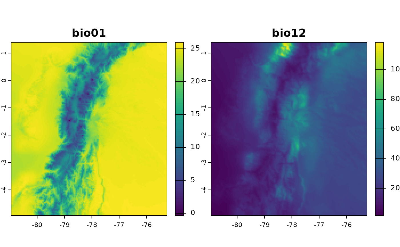
Using Average Temperature as Input
The fastbioclim package also offers the option to use
average temperature (defined with the tavg parameter) for
calculating bioclimatic variables.
# Average temperature
tavg_ecu <- system.file("extdata/ecuador/", package = "egdata.fastbioclim") |>
  list.files("tavg", full.names = TRUE) |> rast()
# Define the directory where the rasters will be saved
output_dir_bioclim_v2 <- file.path(tempdir(), "bioclim_ecuador_v2")

bioclim_ecu_v2 <- derive_bioclim(
  bios = 1:19,
  tavg = tavg_ecu,
  tmin = tmin_ecu,
  tmax = tmax_ecu,
  prcp = prcp_ecu,
  output_dir = output_dir_bioclim_v2,
  overwrite = TRUE
)
# Difference between bio01s when tavg is used
plot(bioclim_ecu_v2[["bio01"]] - bioclim_ecu[["bio01"]])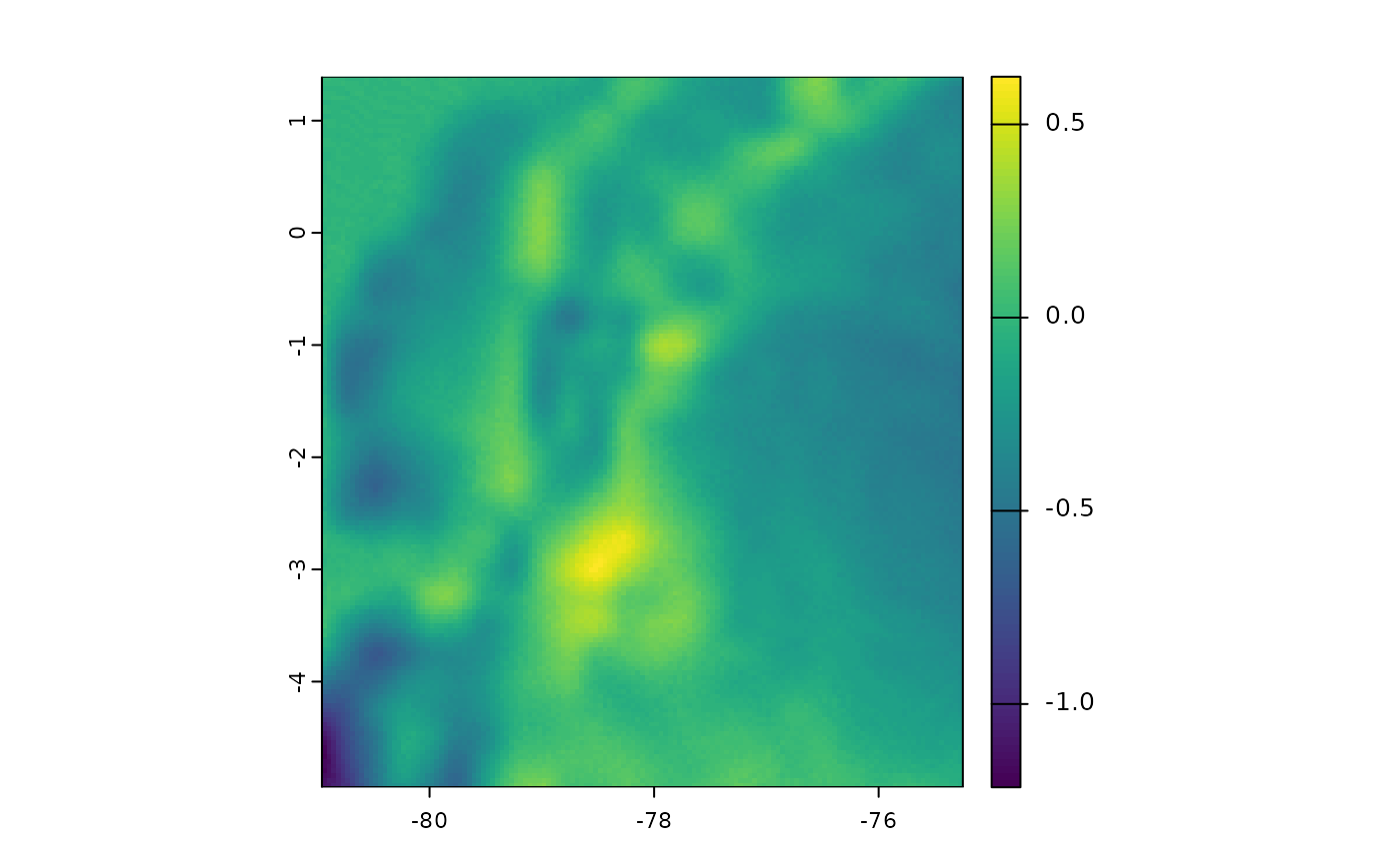
Selecting a Subset of Variables
Often, it is not necessary to use all bioclimatic variables in our
analyses. For this reason, and unlike biovars(), you can
define in the bios parameter the number that identifies
each of the bioclimatic variables. This way, it is not necessary to
obtain all 19 variables to then select only the variables of interest.
In the following example, only four variables will be obtained (bio05,
bio06, bio13, and bio14). This example is somewhat faster, as it is not
necessary to internally calculate the warmest/coldest or driest/wettest
quarters.
bios4_ecu <- derive_bioclim(
  tmin = tmin_ecu,
  tmax = tmax_ecu,
  prcp = prcp_ecu,
  bios = c(5, 6, 13, 14),
  overwrite = TRUE
)
plot(bios4_ecu)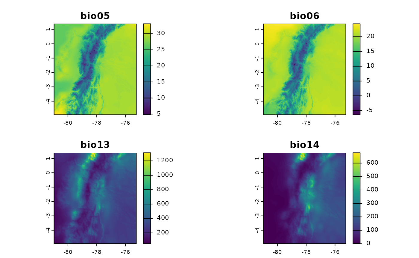
Building Summaries with Other Variables
Another important functionality of fastbioclim is the
option to obtain statistics similar to bioclimatic variables but with
other variables. As an example, we will create summaries of average
monthly wind variables. For the quarterly interactive variables, we will
use the wettest and driest quarters.
wind_ecu <- system.file("extdata/ecuador/", package = "egdata.fastbioclim") |>
  list.files("wind", full.names = TRUE) |> rast()
wind_dir_ecu <- file.path(tempdir(), "wind_ecuador")

ecu_stats <- derive_statistics(
  variable = wind_ecu,
  stats = c("mean", "max", "min", "stdev", "max_period", "min_period"),
  inter_variable = prcp_ecu,
  inter_stats = c("max_inter", "min_inter"),
  output_prefix = "wind",
  suffix_inter_max = "wettest",
  suffix_inter_min = "driest",
  overwrite = TRUE,
  output_dir = wind_dir_ecu
)
plot(ecu_stats)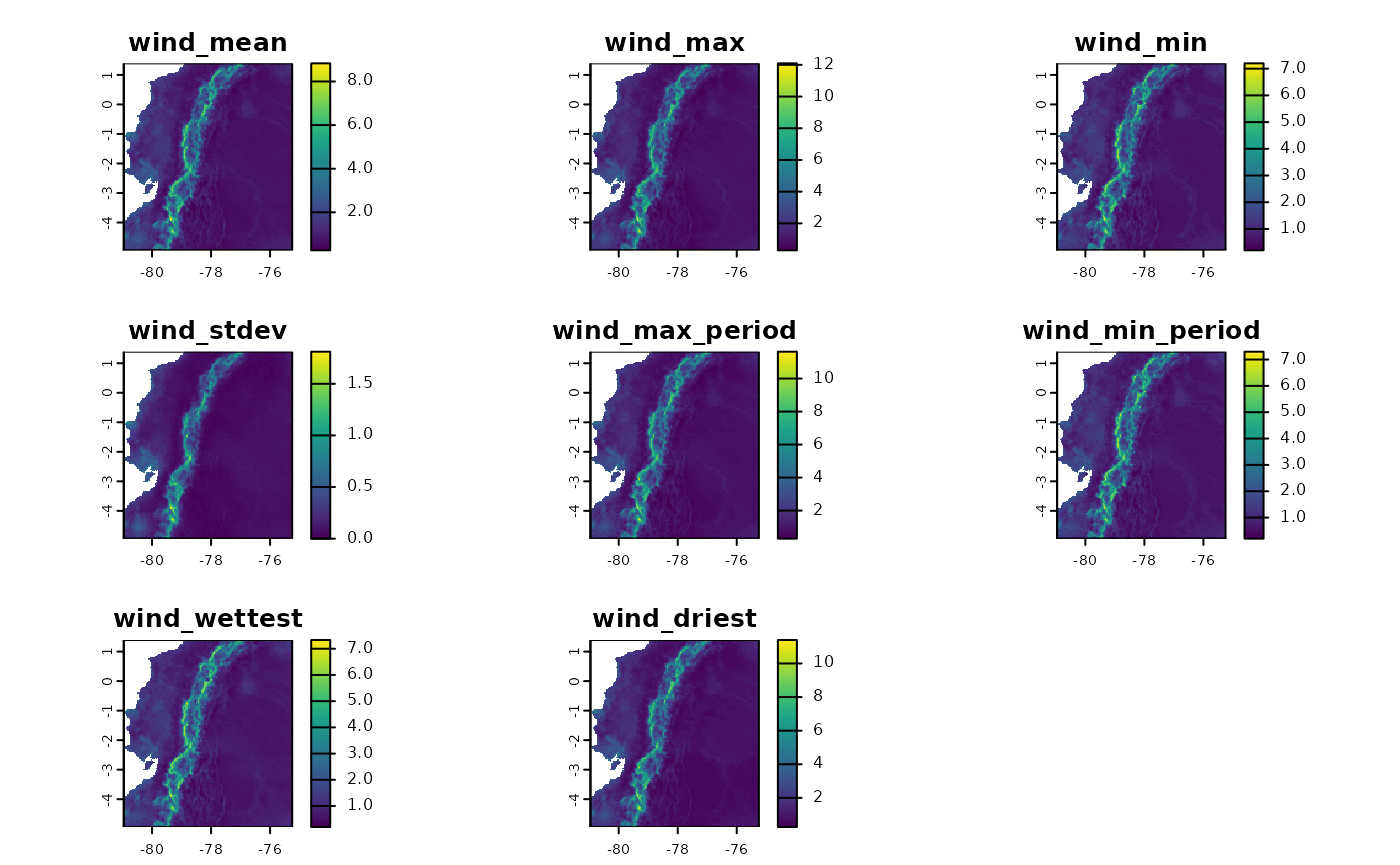
Subsets of variables can also be constructed. In this case, we will create wind variables, but only based on the interaction with temperature, which correspond to “Wind in the warmest quarter” and “Wind in the coldest quarter”.
ecu_stats_v2 <- derive_statistics(
  variable = wind_ecu,
  stats = NULL,
  inter_variable = tavg_ecu,
  inter_stats = c("max_inter", "min_inter"),
  output_prefix = "wind",
  suffix_inter_max = "warmest",
  suffix_inter_min = "coldest",
  overwrite = TRUE,
  output_dir = wind_dir_ecu
)
plot(ecu_stats_v2)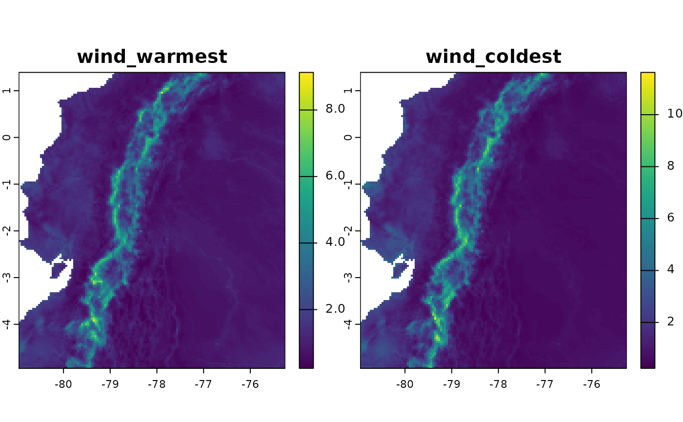
Building for the Neotropics: 35 Variables
Based on the ANUCLIM 6.1 nomenclature (Xu & Hutchinson, 2012),
derive_bioclim() also offers the option to create
bioclimatic variables based on moisture and solar radiation indices. In
this case, we will construct the 35 bioclimatic variables for an extent
covering the Neotropics.
For this case, the “auto” method should use the “tiled” method for
creating the variables. But you can also force it to use this method
with the parameter method="tiled". This method will divide
the area of interest into tiles using the decimal degrees defined in the
tile_degrees parameter (5 is the default value).
Parallelization: It is also important to mention
that the ‘tiled’ method can be parallelized using
future::plan(). For more information, consult the
documentation of that package.
Progress Bar: A progress bar is available using the
progressr package. To activate it, you need to use the
function progressr::handlers() or
progressr::with_progress(). For more information, consult
the documentation of that package.
# Get a list of rasters and create a SpatRaster for each variable
# Average temperature
tavg_neo <- system.file("extdata/neotropics/", package = "egdata.fastbioclim") |>
  list.files("tavg", full.names = TRUE) |> rast()
# Minimum temperature
tmin_neo <- system.file("extdata/neotropics/", package = "egdata.fastbioclim") |>
  list.files("tmin", full.names = TRUE) |> rast()
# Maximum temperature
tmax_neo <- system.file("extdata/neotropics/", package = "egdata.fastbioclim") |>
  list.files("tmax", full.names = TRUE) |> rast()
# Precipitation
prcp_neo <- system.file("extdata/neotropics/", package = "egdata.fastbioclim") |>
  list.files("prcp", full.names = TRUE) |> rast()
# Solar radiation
srad_neo <- system.file("extdata/neotropics/", package = "egdata.fastbioclim") |>
  list.files("srad", full.names = TRUE) |> rast()
# Climatic moisture index
mois_neo <- system.file("extdata/neotropics/", package = "egdata.fastbioclim") |>
  list.files("cmi", full.names = TRUE) |> rast()

# Define the directory where the rasters will be saved
output_dir_neo <- file.path(tempdir(), "bioclim_neotropics")

# Activate progress bar
# progressr::handlers(global = TRUE)

# Define parallelization plan
# future::plan("multisession", workers = 4)

# Get the 35 variables for the Neotropics
bioclim_neo <- derive_bioclim(
  bios = 1:35,
  tavg = tavg_neo,
  tmin = tmin_neo,
  tmax = tmax_neo,
  prcp = prcp_neo,
  srad = srad_neo,
  mois = mois_neo,
  method = "tiled",
  tile_degrees = 20,
  output_dir = output_dir_neo,
  overwrite = TRUE
)
print(bioclim_neo)
## class : SpatRaster
## size : 2120, 1978, 35 (nrow, ncol, nlyr)
## resolution : 0.04166667, 0.04166667 (x, y)
## extent : -117.1251, -34.70847, -55.60847, 32.72486 (xmin, xmax, ymin, ymax)
## coord. ref. : lon/lat WGS 84 (EPSG:4326)
## sources : bio01.tif
## bio02.tif
## bio03.tif
## ... and 32 more sources
## names : bio01, bio02, bio03, bio04, bio05, bio06, ...
## min values : -15.087239, 0.069661, 1.224817, 5.000592, -6.597656, -26.5, ...
## max values : 30.276041, 18.902475, 91.69207, 836.565613, 42.875, 26.296875, ...Example with a User-Defined Region
Another useful parameter in the fastbioclim package is
the option to provide an ‘sf’ object to delimit and mask an area of
interest. The calculation of the bioclimatic variables will only be
performed in this area.
# Get areas of interest
mex <- qs2::qs_read(system.file("extdata/mex.qs2", package = "egdata.fastbioclim"))
# Get only bio10
bio10_mex <- derive_bioclim(
  bios = 10,
  tmax = tmax_neo,
  tmin = tmin_neo,
  user_region = mex,
  overwrite = TRUE,
  output_dir = file.path(tempdir(), "bio10_mex")
)
plot(bio10_mex)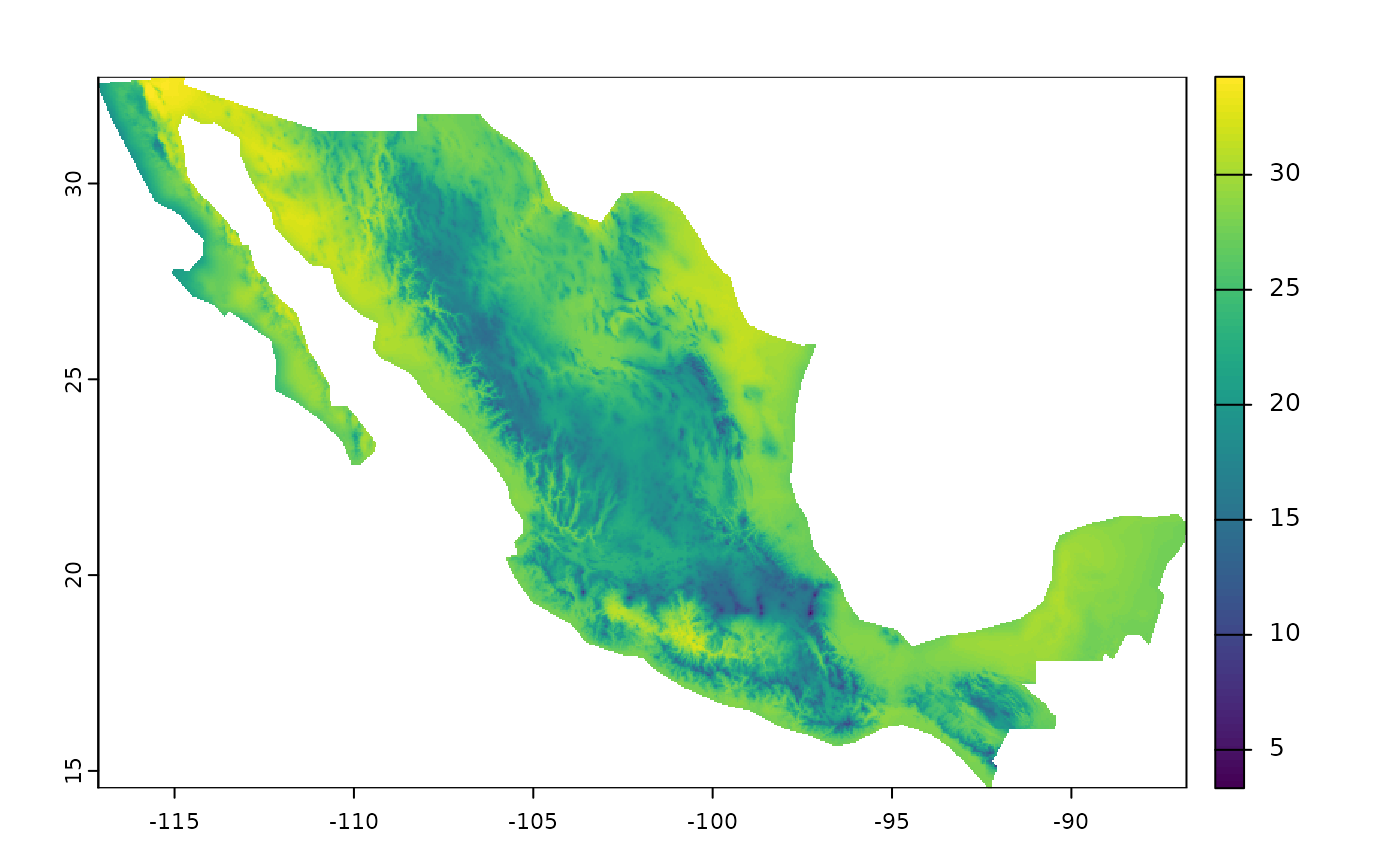
Example with a Static Variable
An advanced option within the package is the ability to determine static variables for the maximum and minimum variables by months (or units) and periods. This can be useful if the research questions are related to a specific time (e.g., seasons of the year) or in the construction of time series.
In this case, we will create the bio10 variable in Mexico again, but
using the quarter of June, July, and August as a reference. To do this,
we must create a SpatRaster that defines the period of interest. In
fastbioclim, the reference is always the first month of the
period or the unit. In this case, that month corresponds to the number
6. Therefore, we will create a raster filled with this number, to then
be used as a reference in the creation of the ‘bio10’ variable.
# Create a raster of 6s for the Neotropics
warmest <- tavg_neo[[1]]
warmest[!is.na(warmest)] <- 6
names(warmest) <- "warmest_period"
# Important: For the 'tiled' method, rasters must be saved to disk
terra::writeRaster(warmest, file.path(tempdir(), "warmest_static.tif"), overwrite = TRUE)
warmest <- terra::rast(file.path(tempdir(), "warmest_static.tif"))
plot(warmest)
# Get only bio10
bio10_war <- derive_bioclim(
  bios = 10,
  tmax = tmax_neo,
  tmin = tmin_neo,
  user_region = mex,
  warmest_period = warmest,
  overwrite = TRUE,
  output_dir = file.path(tempdir(), "bio10_war")
)
# Differences in bio10 for Mexico
plot(bio10_mex - bio10_war)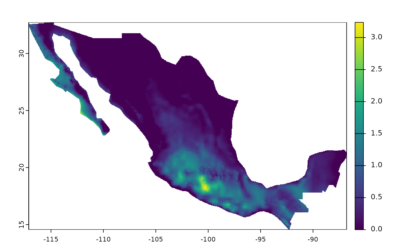
Citation
If you use fastbioclim in your research, please cite our software note:
Pinilla‐Buitrago, G. E., & Osorio‐Olvera, L. (2026). fastbioclim: An R package for creating custom‐time bioclimatic and derived environmental summary variables. Methods in Ecology and Evolution., 17(5), 1585-1594. doi:10.1111/2041-210x.70291
To get the most up-to-date citation format from within R, you can always run:
citation("fastbioclim")