Trinary Maps Vignette

Background

Continuous model predictions are compared against binary data for evaluation in a variety of application; I’m thinking about Species Distribution Models (SDMs) but the following could be probably be used for any application. To evaluate the continuous predictions of the model - in the SDM case the ‘suitability’ scores - one must choose a threshold value of suitability above which the model predicts a species presence and below which the model predicts absence. Coming up with a reasonable threshold is difficult for SDMs, particularly when presence-backround data are involved. Use of the AUC statistic is meant to avoid the issues of choosing a particular threshold and evaluate model performance over all possible thresholds. Even still, in SDM applications, there is still often a need for generating a binary map from continuous predictions, which means picking a threshold.

The specific problem of choosing a threshold when using presence-background data for SDMs is that the background is ‘contaminated’ - it contains (unknown) presences that biases binary classification statistics. One common threshold choice is based on maximizing the sum of sensitivity and specificity (i.e., the Youden threshold), but this penalizes a model for incorrectly predicting background points as presence locations, when in fact they may be presences.The contribution of ‘trinaryMaps’ is to put some useful bounds on what reasonable values of the threshold might be. If we can’t determine an optimal threshold, we can at least identify upper and lower limits so we know we have it surrounded.

The approach to identifying these limits is heuristic and not based on any formal theory; rather it is based on analyzing the ROC curve and identifying limits beyond which model predictions aren’t likely to be very useful in the application of SDMs. For example, why would any care about the discrimination of an SDM based on a threshold that gets only 7% of presences correct? This implies there should be a upper limit on a useful threshold (higher threshold implies fewer predicted presences). Similarly, why would anyone want a model that predicts that only 4% of the background is an absence? If your model were that non-discriminating, why even build a model when you could just use the modeling domain as a range estimate? So this suggests there is a useful lower limit (lower threshold implies more predicted presences). How can we objectively find these upper and lower limits? Answering that is the contribution of trinaryMaps.

Using Trinary Maps

Building trinary maps involves the same inputs as one would use for binary classification and in this package is specifically structured for use with SDMs: 1. Model prediction (spatRaster) 2. Occurrences coordinates (data.frame) 3. Background coordinates (data.frame)

Basic Workflow

The trinaryMapWorkflow() function is the main entry point for using the package. It performs the following steps: 1. Calculates upper and lower ROC bounds 2. Creates a trinary map based on these bounds 3. Calculates range sizes associated with the generated trinary map 4. Plots the ROC curve with upper and lower ROC bounds.

Here’s an example of how to use the trinaryMapWorkflow function:

library(trinaryMaps)
library(terra)

## terra 1.8.10

# YOU CAN REGENERATE THE OCCURRENCE, BACKGROUND AND RASTER PREDICTION OF 
# THIS EXAMPLE USING THE CODE AT THE END OF THIS VIGNETTE
ext_data <- system.file("extdata", package = 'trinaryMaps')

occs <- read.csv(paste0(ext_data, "/occs.csv"))
bg <- read.csv(paste0(ext_data, "/bg.csv"))
r <- terra::rast(paste0(ext_data, "/prediction.tif"))
# Run trinaryMapWorkflow
tr <- trinaryMapWorkflow(pres = occs, 
                         background = bg, 
                         rModel = r)

## 94 presences and 9681 background points used for building trinary maps

Plotting the Trinary Map

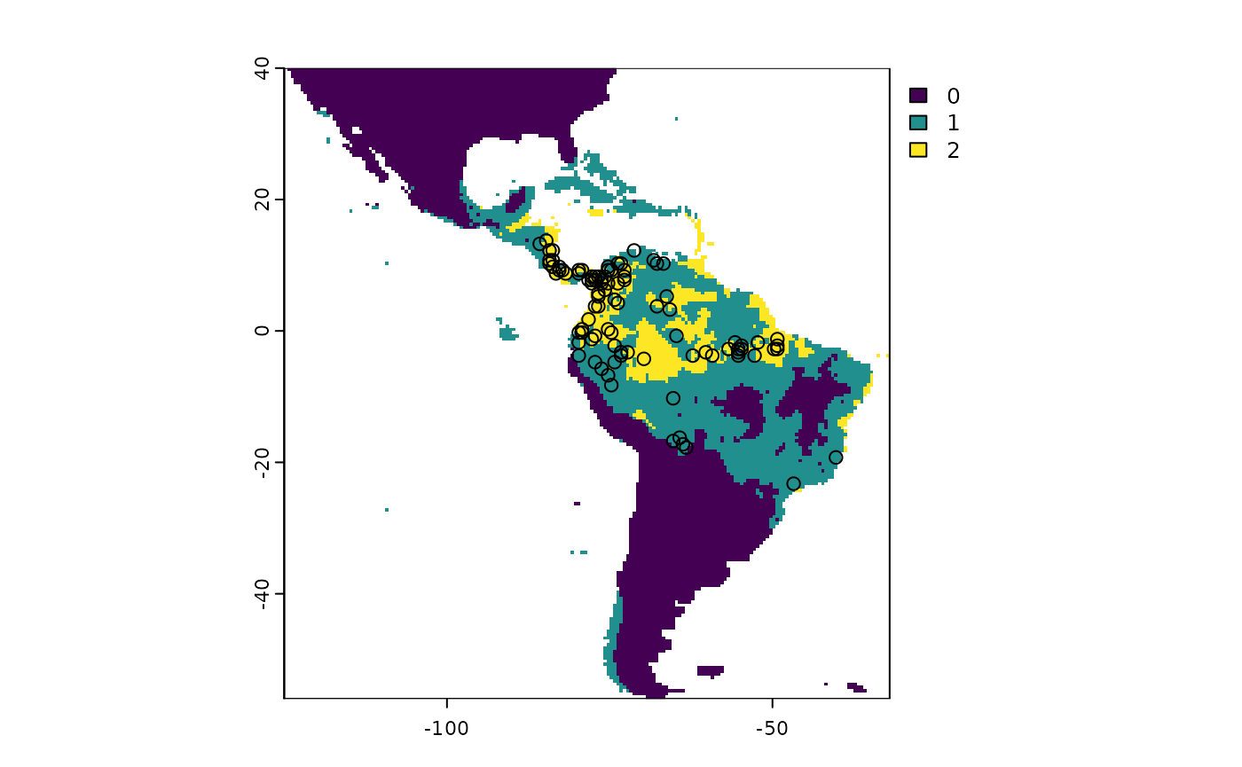
The trinary map is a categorical map that has been transformed into three classes based on the upper and lower bounds calculated by the trinaryMapWorkflow() function. This plot provides a visual representation of where the three classes occur. Class 0 corresponds to pixels with values below the higher ROC bound threshold (definitely unoccupied habitat), class 1 correspond to pixels greater or equal to the upper ROC bound threshold but less than the lower ROC bound threshold (marginal, occasional, or uncertain occupied habitat), and class 2 denotes pixels with values above the lower ROC bound threshold (likely occupied habitat).

plot(tr$trinary.rasters)
points(occs)

Range Size

This chunk calculates the range sizes associated with each threshold value in the trinary map. The range size is an important metric that can be used to understand the sensitivity and specificity of the model predictions at different threshold values.

# Area
trinaryRangeSize(tr$trinary.rasters)

##   range.size.lo.km2 range.size.hi.km2
## 1          13413279           3385016

Trinary Map ROC Plots

The function trinaryROCPlot() generates five ROC plots that help determine the lower and upper bound thresholds. These plots facilitate understanding of how the trinary map is constructed.

ROC

This plot shows the smoothed ROC curve by binormal or density smoothing. The red dot marks the location of the lower ROC bound threshold, which represents the minimum sensitivity and maximum specificity value. The yellow dot indicates the youden threshold, corresponding to the maximum sum of sensitivity and specificity values. The blue dot marks the upper ROC bound threshold, which represents the maximum sensitivity and the minimum value on specificity.

ROC’: First Derivative

The first derivative of the smoothed ROC curve is shown here. This plot helps identify the point on the ROC curve where the trade-off between true positive rates and false positive rates is optimized. Note that the youden threshold corresponds to the root.

logmod(ROC’’): Logmod of Second Derivative

This plot displays the second derivative of the smoothed ROC curve after applying a logmod transformation. It helps to identify the upper ROC bound threshold (blue).

Inverted ROC

To calculate the upper bound threshold, the horizontal and vertical axes are inverted in this plot. This results in an “inverted ROC” curve where high specificity values correspond to low true positive rates, and vice versa.

logmod(Inverted ROC)

The second derivative of the inverted ROC curve is calculated after applying a logmod transformation. The red dot marks the lower ROC bound threshold.

trinaryROCPlot(tr$threshs$plotThings, trinaryDF = tr$threshs$trinaryDF)

Custom example (trinaryROCRoots) GEPB [2025-01-21]: NOT WORKING. Waiting for Cory´s reply e-mail (2024-08-25)

The trinaryMapWorkflow() function calculates the upper and lower ROC bounds using default parameters. If you want to customize the calculation of both bounds, you can modify the following parameters:

maxTPQuantile: A quantile value representing the predicted values at presence locations used to determine the upper ROC threshold for presence predictions. For example, a value of 0.3 means the function uses the 30th percentile of the predicted presence values as the upper threshold, ensuring that the model maintains at least 70% sensitivity.
sdMultiplier: A scaling factor applied to the standard deviation of the predictions, used inconjunction with max.sens to calculate the lower ROC bound.
max.sens: The maximum true positive rate allowed for the lower ROC bound calculation. This parameter is used in combination with sdMultiplier to determine the optimal threshold for the lower bound.

Here, we will modified the maximum quantile to 20th percentile, and change the maximum sensitivity allowed for the lower ROC bound to 0.99.

# Issues with maxTPQuantile, max.sens, and sdMultiplier. Results are the same that previus example.
tr2 <- trinaryMapWorkflow(pres = occs, 
                          background = bg, 
                          rModel = r, 
                          maxTPQuantile = 0.01,
                          max.sens = 0.01)

## 94 presences and 9681 background points used for building trinary maps

plot(tr2$trinary.rasters)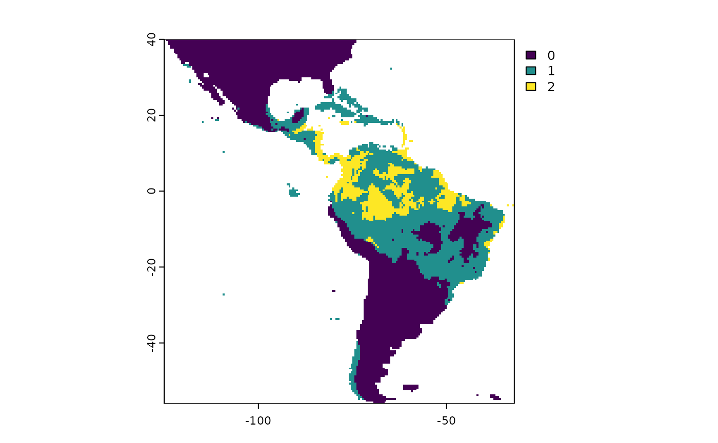

trinaryROCPlot(tr2$threshs$plotThings, trinaryDF = tr2$threshs$trinaryDF)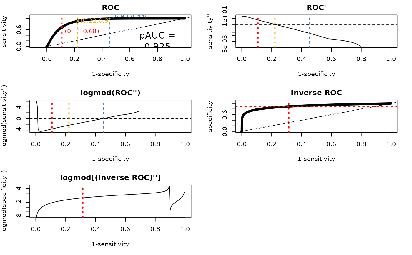

Additional Code

library(predicts)
library(maxnet)
# Load example data
occurence <- system.file("/ex/bradypus.csv", package = "predicts")
occ <- read.csv(occurence)[, -1]
f <- system.file("ex/bio.tif", package = "predicts")
envs <- terra::rast(f)

# Prepare data for modeling
data <- terra::values(envs) |> as.data.frame()
data$ID <- 1:(terra::nrow(envs) * terra::ncol(envs))
occs.p <- terra::extract(envs, occ, cells = TRUE)
data$p <- rep(0, terra::ncell(envs))
data$p[occs.p$cell] <- 1
data$x <- terra::xFromCell(envs, 1:terra::ncell(envs))
data$y <- terra::yFromCell(envs, 1:terra::ncell(envs))
data <- na.omit(data)

# Build and predict model
mod <- maxnet(data$p, data[, 1:9])
p.vals <- predict(mod, terra::values(envs), type = "cloglog")
suitability <- rep(NA, terra::ncell(envs))
suitability[data$ID] <- p.vals
r <- envs[[1]]
names(r) <- "suitability"
terra::values(r) <- suitability
occs <- data[data$p == 1, c("x", "y")]
bg <- data[data$p == 0, c("x", "y")]

Cory Merow and Gonzalo E. Pinilla-Buitrago

2024-08-31